
By Zachary G. Nicolaou
Welcome to another academic year, AMATH! It’s summer as I’m writing, and Lewis has been quiet these days, hopefully implying that everyone is enjoying the weather. I’ve been holding down the fort on the first floor and admiring Facilities' progress; we will be prepared for a fire when everyone returns. Congrats to the students and faculty for raising appropriate concerns about building safety and the leadership for taking concrete measures! The isolation has been nice as I’m trying to wrap up old projects, but it will be great to see activity return soon.
For a quick background, I’m midway through my third year as an Acting Instructor and WRF postdoc in the department. I have had the pleasure of advising several excellent undergraduate, Master’s, and Ph.D. students in the department on research projects. My research focuses on symmetry, pattern formation, and the development of complexity in dynamical systems, and I collaborate with Nathan Kutz and Steve Brunton at the AI Institute in Dynamic Systems. I’ve also enjoyed working on the Diversity Committee in the department for the last two years. The committee oversees many endeavors, which I want to encourage students to take advantage of. These include the Women in Applied Mathematics Mentorship (WAMM) program, the annual department climate orientation and check-in events, the department’s public diversity plan, and a variety of cultural social events. The committee operates on student member labor and we can always use more help, so I encourage you to reach out to us if you want to contribute to the department’s efforts!
I do quite a bit of coding, both for my own work and as one of the maintainers of the PySINDy package that Nathan and Steve’s students created [1]. Just a few years ago, the way to integrate an ODE was to walk to the library, check out a reference book [2], and copy an algorithm by hand. I remember very well debugging a molecular dynamics program for my first undergraduate research for hours only to discover a missing digit in 92097/339200 (one of those Runge-Kutta magic parameters). Nowadays, things are a little different, with extensive and well-tested Python packages like numpy and scipy that hide away many details for convenience, and you can reliably integrate a complex system with just a couple of lines of code. But in other ways, not much has changed. If you spend enough time in numerics, you may find that you need to delve into the core of the algorithms to make progress.
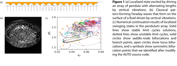
To illustrate, I’ll tell you some about ongoing work on localized states in a pendulum array [Figure 1(a)], which I’ve been studying recently in collaboration with former AMATH Acting Instructor Jason Bramburger (now an assistant professor at Concordia University and a brand new father). Just before starting at UW, I studied the classical pattern-forming Faraday waves [Figure 1(b)], which form on the surface of a liquid when driven by vertical vibrations. I was interested in the impact of heterogeneous geometries, and, to simplify the problem, I had introduced the alternating pendula array model [3]. Besides interesting quasiperiodic behavior [4], we found unexpected localized swinging states that result from random initial conditions for certain parameter values. Fortunately for me, I was joining a department with one of the rising experts on localized states (Jason), so we chatted a bit before he started his new position. Jason suggested there may be a connection with so-called snaking bifurcations that give rise to localized states in the Swift Hohenberg [5], so I set out to resolve the question numerically.
I won’t spend too long trying to describe numerical continuation [6], but I should try to explain a little. We are given a dynamical system like x=fx;μ, which depends on a parameter , like the driving amplitude ad in our pendulum system. We know a solution for a given μ=0, say a steady state 0=f(x0,0). The goal is to determine how that solution will vary with . The foundational result is the implicit function theorem, which guarantees the existence of a unique solution branch such that 0=f(x*; μ) for near 0 with x*0=x0, provided the Jacobian matrix Jij=fixj is nonsingular. The real parts of the eigenvalues of the Jacobian determine the growth rates of perturbations, so values of where the real part of an eigenvalue changes sign indicate changes in stability. Such points are called bifurcation points, and the implicit function theorem can break down there. Fortunately, even at such points, it is usually possible to continue solution branches by taking advantage of local analysis. If, for example, a single real eigenvalue passes through zero at x*c=xc and the leading term in the Taylor series expansion of fx;μaround (xc;c) does not vanish, the bifurcation point is a saddle-node bifurcation, and the solution branch simply turns around at a limit point that looks locally like xc±cμ-c. If the leading term of the Taylor series does vanish, multiple solution branches can come together in transcritical or pitchfork bifurcations, but these “branch points” are non-generic in the sense that they break apart under small perturbations to the dynamical equations, which generically alter the leader-order Taylor series coefficient.
Numerical tools have been developed since the seventies to continue solution branches and even switch branches at branch points, mapping out a bifurcation diagram that can give valuable qualitative information about the system. I’d heard of a legacy FORTRAN package called AUTO [7], and I hoped to be able to use it to answer Jason’s question about the relationship between the localized states in the pendula and the Swift-Hohenberg equation. I had already been using AUTO before I came to UW, so it was amusing to realize that Nathan used it extensively for his Ph.D. thesis a few years back [8].
Figure 1(c) shows the results of our AUTO continuation for the localized states of the pendulum array. We found that the bifurcations of localized states in the pendulum array do not follow the snaking bifurcations of the Swift-Hohenberg equation, but more closely resembled strange attractors and heteroclinic tangles of chaotic systems. How can we rationalize this behavior? I mentioned before the non-genericity of transcritical and pitchfork bifurcations. The reason we care about such non-generic behavior is that the systems we study often have symmetries that ensure the existence of non-generic bifurcation points. The pendulum array, for example, has reflectional and translational symmetries, and such branch points do occur in the continuation (marked with solid dots in Fig. 1c). AUTO finds these points by detecting when the determinant of the Jacobian changes sign, but, as we discovered, other kinds of non-generic behavior can also occur in the eigenvalues of symmetric systems. Rather than a single real eigenvalue with a vanishing leading-order Taylor term, it’s possible for two real eigenvalues to simultaneously vanish in symmetric systems, and AUTO will not detect such bifurcations since the sign of the determinant of the Jacobian will not change there. Detecting these points required learning a bit of FORTRAN (not as bad as it sounds) and delving into the source code to modify the bifurcation detection. By adding just a handful of lines, we were able to identify these symmetric bifurcation points (marked with x’s in Fig. 1c) and recognize their organizing role in the symmetry breaking leading to localization. Do we totally understand the mechanism now? By no means. We haven’t even finished the paper yet (and my deadline is approaching in just a few weeks…). But we’ve made a step in the analysis that wasn’t possible with the existing software.
I should wrap up--what’s the point? Just some advice: take advantage of existing software, but try to recognize its limitations and take a peek under the hood if you need to. Despite the appeal of a black box solution, scientific progress may necessitate reading old papers, understanding the code you use, and making changes.
References
[1] Kaptanoglu et al., PySINDy: A comprehensive Python package for robust sparse system identification, J. Open Source Softw. 7, 3994 (2021).
[2] Press, Teukolsky, Vetterling, and Flannery, Numerical Recipes: The Art of Scientific Computing (Cambridge University Press, New York, 1986).
[3] Nicolaou, Case, van der Wee, Driscoll, and Motter, Heterogeneity-stabilized homogeneous states in driven media, Nat. Comm. 12, 4486 (2021).
[4] Nicolaou and Motter, Anharmonic classical time crystals: A coresonance pattern formation mechanism, Phys. Rev. Research 3, 023106 (2021).
[5] Burke and Knobloch, Localized states in the generalized Swift-Hohenberg equation, Phys. Rev. E 73, 056211 (2006).
[6] Keller, Lectures on numerical methods in bifurcation problems, Appl. Math. 217, 50 (1987).
[7] Doedel, Keller, and Kernevez, Numerical analysis and control of bifurcation problems (I): bifurcation in finite dimensions, Int. J. Bifurcat. Chaos 1, 493-520 (1991).
[8] Kutz, Pulse propagation in nonlinear optical fibers using phase-sensitive amplifiers, Northwestern University, 1994.